Seconds behind

The common instruction for keeping a safe distance behind another vehicle is to stay 2 seconds behind it (I don't think it's actually a law, at least not in Ontario -- correct me if I'm wrong). The common method for calculating this is to look for a large object on the side of road, ahead of the car in front of you, wait until that car passes the object, then count the number of seconds until you pass it. If it's less than 2 Mississippis, you're too close.

I've tried this a few times. It's not quite satisfying. First off, it requires some low grade distracted driving. I should be paying attention to road, especially the car ahead of me, as well as other cars around me and the traffic signs, but instead I'm counting as I watch things pass by on the side of the road. Because of this divided focus, the method is also prone to inaccuracy.

After having seen enough accidents that were almost certainly made worse because drivers were following too closely and read about a few more, I became curious what the actual safe distances were. If I am driving at a certain speed behind another car driving the same speed, exactly how many metres does a 2 second gap translate to?

The instruction is common enough that I figured I should be able to Google it and find these values for some common speed limits. All I found was the same instruction, whether from government transportation agencies or driving enthusiasts. No values were given, just the same method for computing them, if anything.

There is another method we can use, though: math. In particular, the kind I learned in high school chemistry class, namely dimensional analysis. Using this technique, it's pretty easy to convert from kilometres per hour to metres per second (details below). Multiply by 2 seconds and you get the distance.

In Canada, the speed limits typically run from 40 km/hr to 120 km/hr (typically on the 10s). These speed limits, their equivalents in metres per second, and the resulting safe minimum distances are summarized in the following table (rounded to the nearest 10th).

km/hr	m/sec	metres behind
40	11.1	22.2
50	13.9	27.8
60	16.7	33.3
70	19.4	38.9
80	22.2	44.4
90	25.0	50.0
100	27.8	55.6
110	30.6	61.1
120	33.3	66.7

Here's a similar chart for imperial measurements, with miles in places of kilometres and feet instead of metres.

miles/hr	feet/sec	feet behind
20	29.3	58.7
25	36.7	73.3
30	44.0	88.0
35	51.3	102.7
40	58.7	117.3
45	66.0	132.0
50	73.3	146.7
55	80.7	161.3
60	88.0	176.0
65	95.3	190.7
70	102.7	205.3
75	110.0	220.0
80	117.3	234.7

Having these numbers isn't the perfect solution to knowing how far back to to stay behind other vehicles either. It's not like we can get out and measure while we're driving, and I don't think we're great judges of distance, especially when we're driving. Nevertheless, I think it can still be informative.

For example, suppose we are driving at the lowest speed on the first chart (the typical speed through a school zone in Ontario). The bumper to bumper length of a Honda Accord, a mid-sized sedan, is a little under 5 metres. At that speed, the space between me and the car in front of me should be at least big enough to fit an Accord, and there should be plenty of room to fit another in front and another behind (of course, it may be difficult to manoeuvre those cars into that space at that speed, and if we do, we're well out of the realm of safe distances).

A highway speeds (100 to 120 km / hr), the numbers are more than double that. The gap between cars should be larger than the length of an Olympic sized swimming pool. And yet, it's not uncommon to see cars on the highway driving so close that there isn't room enough for a single car between. In other words, people aren't even keeping the safe distance that is supposed to be used in a school zone.

I was pretty surprised to see these numbers. I generally thought I was keeping safe distances. It's certainly true that most of the time I'm keeping a safer distance than a lot of vehicles I encounter. But it's clear, after doing the calculations, that I'm not keeping as far back as I should be.

There is a third option to consider for calculating safe distances. Don't require drivers to do it themselves. The required technology has been around for a long time. Though I expect it will be an essential component of self-driving cars, it's rarely been applied to cars human-driven cars.

------

There are 1000 metres per kilometre, 60 minutes per hour, and 60 seconds per minute. If we are driving X kilometres per hour, that works out to $(X km / hr) \times (1000 m / km) \times (60 min / hr) \times (60 sec / min) = (1000/3600)\times X m / sec = (5/18)\times X m / sec.$

The calculations for feet per second are similar, with 5280 feet per mile in place of 1000 metres per kilometre, yielding
$(X mi / hr) \times (5280 ft / mi) \times (60 min / hr) \times (60 sec / min) = (5280/3600)\times X ft / sec = (22/15)\times X ft / sec.$

Friends in high density places

Last August, I found the map below.  2% of the Australian population lives in the yellow area and the remaining 98% lives in the white area.

Like Australia, Canada is geographically large, but sparsely populated.  Canada's population density is a little higher, though not by much.  On average, there are 3.56 people per square kilometre in Canada compared to Australia's 3.06.  Also, like Australia, our population is centred around a small number of urban areas.  The three most populous metropolitan areas, Toronto, Montreal, and Vancouver, alone make up more than a third of our population, the top 10 more than a half, and the top 100 nearly 80% (mind you, most of the cities in that top 100 list have less than 100,000 people, and some, such as Timmins and Cape Breton are quite large in area).  (Population data culled from various Wikipedia pages).

So I wondered what a similar map for Canada would look like.

Unfortunately, there doesn't seem to be much information out there about how the map was created.  Within each of the yellow and white areas, we see other borders drawn in.  I'm assuming that these represent some national subdivisions, perhaps municipal boundaries or census regions.  So whoever made the map made a choice of which regions to colour yellow and which regions to colour white.

There are many choices that would split the population between 2% and 98%, though.  For example, to construct a region containing 98% of the population, like the one coloured white here, one could start with the sparsely populated inland regions and add increasingly denser regions until 98% is reached.  The result would not be very interesting.  Australia's population is roughly 23.5 million.  2% of that is 470,000, only a bit smaller than the population of Tasmania, the country's smallest province, and roughly 10% of the population of Sydney's, the country's largest city.

So we could create a map where all of Australia other than some parts of Tasmania are coloured white, or where all but a few urban specks of Sydney are coloured white.  In the latter case, the yellow parts would probably so small that it would be difficult or impossible to see them.  The map would hardly be different from a plain map of Australia.  What makes the existing map interesting, though, is how small the area containing 98% of the population is.

To make the map as interesting as possible, then, we would want the white part to be as small as possible.  As I said above, however, there is no information about how the map was created.  Is the white region as small as it could be, based on the subdivisions used, or is there something other choice that would lead to an even smaller region?  Did the creator simply pick the $m$ sparsest or least populous subdivisions, or was something more sophisticated used?

I found it through Twisted Sifter, which refers back to a Reddit thread.  This thread links to an image hosted on imgur, which I embedded above.  After that the trail goes cold.  One of comments from the original poster suggest that he or she is the one who created it, but there is no follow up, and the user's online profile doesn't offer any direction either.

Without knowing, then, we'd have to come up with our own method.  One simple method is to rank the subdivisions by population, and choose the first $m$ that give 98% of the population.  Another would be to rank by area, and choose the first $m$ that give 98% of the population.  A third option would be to rank by density and choose the first $m$ that give 98% percent of the population.  None of these are guaranteed to give the smallest area that includes 98% percent of the population (or, equivalently, the largest area that includes 2% of the population).

Another less obvious way to solve the problem is through a mathematical technique known as linear programming.  We create a function that gives us the area if a certain set of subdivisions is chosen, then we try to maximize the area under the condition that the percentage of the population that lives in the chosen set of regions is less than or equal to 2%. Ideally, we'd be able to insist that the population is equal to 2%, but this might not be possible.  For our purposes that shouldn't be a problem, though, since a smaller number than 2% would only further illustrate the sparseness.

Now let's write this in mathematical notation.  Suppose that ${\bf c}$ is a vector where entry $i$ of ${\bf c}$ is the area of subdivision $i$.  Let $A$ be a row matrix where column $i$ of the only row of $A$ is the percentage of the population in subdivision $i$.  Let ${\bf x}$ be a vector of variables where entry $i$ of ${\bf x}$ is the variable $x_i$.  If $x_i=1$ when subdivision $i$ is chosen and $0$ otherwise, then $f({\bf x})$ gives the total area for that choice of subdivisions and $A{\bf x}$ is the corresponding percentage of the population.  Then we want the following

• maximize $f({\bf x})={\bf c}\cdot {\bf x}$ such that
• $A{\bf x}\leq 0.02(=2\%)$ and
• $x_i$ is 0 or 1 for each $i$

This is not exactly an linear programming problem.  The third condition makes it a binary integer programming problem, because each $x_i$ can be one of only two integer values, 0 or 1.  To make it a linear programming problem we replace the third condition with the following

• $x_i\geq 0$ for each $i$.

 This could allow for the possibility that a region is partially included.  That is, only a certain percentage of a region's population counts towards the total percentage.  That means that we also want $x_i\leq 1$, since we can't include more than 100% of a region's population.  In that case, the problem is

• maximize $f({\bf x})={\bf c}\cdot {\bf x}$ such that
• $A{\bf x}\leq 0.02$ and
• $0\leq x_i\leq 1$ for each $i$.

As stated, this is not a linear programming problem.  However, we can easily turn it into one.  Suppose that there are $n$ subdivisions in total.  Let $B$ be the $(n+1)\times n$ matrix whose first row is $A$ and whose remaining $n$ rows is the $n\times n$ identity matrix.  Let ${\bf b}$ be the vector with $n+1$ components whose first entry is $0.02$ and whose remaining entries are all 1.  Then we can rewrite the above as

• maximize $f({\bf x})={\bf c}\cdot {\bf x}$ such that
• $B{\bf x}\leq {\bf b}$ and
• $x_i\geq 0$ for each $i$.

This is now a linear programming problem.  Unfortunately, the solution to the linear programming problem is not what we want, although it has the upside of being easier to solve.  In general, solving a binary integer programming problem is not easy.  So we may be able to solve the linear programming problem and use that to get a good solution to our problem (for example, by rounding), even though it might not be the optimal one.  Note that if we restricted to integer solutions, then we get the binary integer programming problem back.  There are some special cases where integer linear problems are easy to solve.  Perhaps this is one.  (Who knows? Maybe one of the three simple methods I gave above will turn out to be the optimal solution, though I'm sceptical any of them would be.)

Seeing a version of this map for Canada would be most interesting to me, because that's where I'm from and because of the geographical similarities.  But maps of this sort could be interesting for other countries, or cities, provinces or states, continents, or even the whole inhabitable world.  And of course, we need not insist on a split between 2% and 98%.  Perhaps a 50/50 split would be interesting.  Maybe there is some other interesting percentage, such as a percentage $X$ for which $X$ percent of the population lives on $100-X$ of the land (if that number even exists).

If the binary integer programming problem could be solved, it would be a simple (though possibly tedious) matter of collecting the required geographic data and plugging it into some map making software.

Update: After finishing this post, I emailed a colleague of mine who has much more experience in linear programming than me to ask him if he had any insights.  He told me that this is a knapsack problem.  I had heard of this problem before, but only informally, so I didn't clue in that it was a special case of integer linear programming.  Oddly, neither the linear programming nor the integer linear programming Wikipedia pages refer to the knapsack problem, nor does the knapsack page refer to either of the other two.

In any case, this is sort of good news, but only good in the sense of "maybe less bad."  The general binary linear programming problem is NP-hard, whereas the knapsack problem is NP-complete.  NP-hard problems are at least as hard to solve as NP-complete problems.  The reason it's only "maybe less bad" is that there is not currently known whether or not there are efficient algorithms for solving NP-complete problems.  According to the Wiki page on the knapsack problem, though, there are efficient algorithms for finding approximate solutions.  Maybe these would be good enough.  Indeed, our eyes may not be able to discern between the optimal solution and an approximate one.  In that case, I guess it's more or less good news.

Notes:

• For more on linear programming, see here and here or, better yet, pick up a book, such as this one, which was what I first learned about linear programming from.
• I don't currently have the resources at my disposal to do any of the above, but the population density below from Statistics Canada probably gives a rough idea of what the result would be.
  
  

Teaching Math with PowerPoint - a post mortem

I taught a second year linear algebra course in the fall term of the 2013 - 2014 school year.  The first few lectures were review of the prerequisite course.  My normal teaching practice consists almost exclusively of writing on the board when I'm not directly interacting with students.  But I figured that since my students had learned the material already, they didn't need to take notes and I could run through it a little faster than if they were seeing it for the first time.

So I put all of the review notes on PDF Slides (not actually PowerPoint, despite what I wrote in the title), using the Beamer package for LaTeX.  The first week went fairly well, so instead of switching back to my usual practice at the end of the review stage, I decided to to continue using slides.  I didn't intend on using them for the rest of the term, but in the end, that's what I did.

Overall, it was well received by the students.  Direct feedback was positive, and I received no complaints on course evaluations.  One complaint that could have been levelled at me is that the slides were not always perfect.  Sometimes there were typos, for example.  Perhaps the students were content with the corrected versions that I later posted on the course website.

Student performance was consistent with other courses I've taught.  A couple of students, but one was a student who was also doing poorly in other classes, and there were extenuating circumstances to explain the other student's failure. 

It would be irresponsible to draw conclusions about the effectiveness of the practice at this stage, mind you.  It was the first and only time I've taught this course and the first time I've used slides to this extent.  Nevertheless, it went well enough that I plan on doing it again in the upcoming year.

Although the course was far more heavily oriented towards slides than any other time I taught, I still did rely heavily on the blackboard.  I believe it's better to work out examples with the students, so I would only write the examples on the slides, and work out the solutions on the blackboard (often putting the final answer on the slides too, though not always).  

I also made heavy use of Beamer's "pause" command.   That way, I could present the text of a given slide gradually, one line at a time or even one word at a time if I wanted to, rather than all at once.  To some extent, this mimics writing on the board, where the content is revealed chalk stroke by chalk stroke.  I think this makes it easier to absorb.  Rather than trying to take in a whole slide's worth of information, only one line needs to be comprehended at time.  I also think it helps to keep the pace of the lecture from getting too fast, an easy temptation to give into with slides (or overheads, in the olden days).

Switching back and forth between the blackboard and the screen was a bit frustrating at times, since it seems that most classrooms equipped with projectors (which is most classrooms, if not all, these days) are not designed to mix the two methods. 

I taught in three different classrooms for the class.  Each room had a different layout with different upsides and downsides.

One of the classrooms had the projector screen covering up one panel of the chalkboard.  This was okay as long as I could fit everything in the other panel.  Occasionally, I needed both, which meant rolling up the screen and turning off the projector, then, when I'm done with the other panel, pulling the screen down and waiting for the projector to turn back on.  None of these are onerous tasks, but they interrupt the flow of the lecture and use up time.

The other two classrooms had their screen covering the middle of the blackboard, with the edges of the boards still exposed to write on.  In one room, the exposed edges were quite large, about the size of the uncovered panel in the other classroom.  In the other, however, they were fairly narrow.  The annoyance in both cases was that if an example took up more than one board, I had to finish it on the other side where it was hard to see what I had written on the first side because the screen was in the way.

Another issue I had is the fact that screen real-estate is quite limited.  Some things could not be fit onto a single slide.  Something on one slide might refer to something on another slide.  On a blackboard, one can use two different panels for the different things, but there is only one screen.

The other problem I ran into was malfunctioning technology.  In one room, the projector bulb burnt out.  In another, I could not access the network to log in to the computer.  Fortunately, computer services was quick to replace the bulb in the former case, and there was another open classroom with a working projector in the latter case.


If I had my way, each room would be equipped with two, or even three, projector screens, one for the current slide, and the other(s) for showing preceding slides or calling up older results or examples.  There would also be a chalkboard with at least two panels to write on, even when all screens are in use.  Of course, this wouldn't be feasible in all but the largest classrooms, and even if it were, it could end up being the classroom version of The Homer.  I'd settle for an effort on the part of classroom designers to consider that someone might want to use both blackboard and projector at the same time.

Despite the space taken up by the above complaints, they were all fairly minor in the grand scheme of the course.  They don't add up to enough to discourage me from doing it again, looking for places to improve, and maybe thinking about trying it for other courses.

Pythagorean Statistics

Suppose that $X_1$ and $X_2$ are independent random variables such that $X_1+X_2$ is defined.  Let $\sigma_1$ and $\sigma_2$, and $\sigma$ be the standard deviations of $X_1$, $X_2,$ and  $X_1+X_2$ respectively.  Then $\sigma^2=\sigma_1^2+\sigma_2^2$ (the numbers $\sigma_1^2,$ $\sigma_2^2$, and $\sigma^2$ are called the variances of $X_1,$ $X_2$, and $X_1+X_2$ respectively).  This looks very Pythagorean Theorem (PT) like.  In fact, at least one person calls it the Pythagorean Theorem of Statistics (PToS).

In the link, the author gives a proof of the PToS, but the proof doesn't look much like the proof for the PT.  Nevertheless, the similarity is hard to ignore.  So I wonder, is the PToS just the PT dressed up in statistical clothing, or is it merely a coincidence that the similarity exists?

I suspect it's the former, but I don't quite see the connection yet.  The PT is about right triangles in a plane, and I don't see what that plane would be for the PToS, nor what the triangle is, nor why the third side of that triangle should be related to $X_1+X_2$.  The other author doesn't seem to be aware of a connection either, since none of the reasons he gives for calling it the PToS are "because it is the Pythagorean Theorem."

Update:

My initial instinct was to represent $X_1$ and $X_2$ with a pair of orthogonal axes using $(\mu_1,\mu_2)$ as the origin, where $\mu_1$ and $\mu_2$ are the means of $X_1$ and $X_2$ respectively.  If we let $\arrow x_1=(\sigma_1,0)$ and $\arrow x_2=(0,\sigma_2)$, then we could represent $X_1+X_2$ with the line through $(\mu_1,\mu_2)$ with the direction vector  $\arrow x_1+\arrow x_2$.  The length of $\arrow x_1+\arrow x_2$ is $\sigma=\sqrt{\sigma_1^2+\sigma_2^2}.$  Therefore, $\sigma^2={\sigma_1^2+\sigma_2^2}.$  So we get the Pythagorean identity. 

This isn't a geometric proof of the Pythagorean Theorem of Statistics, though.  At best, it is an illustration of the Pythagorean Theorem of Statistics by the Pythagorean Theorem from geometry.  It is perhaps natural to represent $X_1$ and $X_2$ by orthogonal axes.  Representing $X_1+X_2$ by the line in the direction of $\arrow x_1+\arrow x_2$ was forced to make the geometry work.  It's not as natural.  The more natural thing to do is represent $X_1+X_2$ by a third axis orthogonal to both $X_1$ and $X_2$.  Also, I do not see how the statistical theorem would follow from the geometrical illustration.

Competition and the Logistic Distribution

In my recent post on the other bell curves, I wondered if there was some familiar processes underlying the logistic distribution that would parallel coin-flipping for the normal distribution.  I noted there that logistic distribution works better for the ELO rating system than the normal distribution did.

I also noted that the curve that describes the logistic distribution arises from population growth models that account for competition for resources.  The ELO rating system is also used in the context of competition, but for games.  I wondered whether there was something to this.  Was it a mere linguistic coincidence, or was there a deeper connection?

Well, I still don't have a complete answer, but I can see at least one connection between the two scenarios.  In both cases, there is competition for a finite resource.  For the population growth model it is food supply, and for games, it is wins. 

The parallel is not exact, however.  In particular, the logistic model is used to describe the size of a population, but for a game, the logistic distribution is only used to compute the probable outcomes within a set of competitors, not the number of competitors. So the connection is not complete.

Understanding Self-Information

I've never taken a course in information theory, but recently I've been trying to learn more about it on my own.  I reached a satisfactory understanding of most of the concepts, but an acceptable understanding of self-information proved elusive for quite a while.  If it were just another term of many, I might have been content to ignore it, but the definitions of all of the other terms rest on this concept, so I didn't consider ignoring it to be an option.

Most introductory texts on information theory that I've seen take the definition as axiomatic.  If an event occurs with probability $p$, then self-information of that event is defined to be $-\log p$, where the logarithm is to some chosen base (often 2).  What I wanted to understand better is why the self-information is defined that way.  In my experience so far, this is rarely explained and never explained well.

It did make some intuitive sense, as various authors claim.  One property of this definition is that the self-information of an event increases as the probability decreases.  This is a reasonable property (I would even say necessary) for any self-information function.  Suppose, for example, that we are playing a game of hangman.  The letter "z" is far less frequent in English than the letter "s", so if a "z" is showing, then it is easier to narrow down the word than it would be if an "s" were showing.  Thus, the rare event "contains the letter 'z'" gives more information than the common event "contains the letter 's'."

But $-\log p$ is not the only function that works like that.  We could also use $1-p,$ which is far simpler and avoids the dreaded logarithms.  Simple is always preferred to complicated, so there must be a reason why $-\log p$ is the function of choice.

Well, in order for information to be transmitted, there must be some way to represent it.  Spoken languages use sounds.  Written languages use words with letters some alphabet.  Computers use strings of 0s and 1s, which we could think of as words from a two letter alphabet. 

The number of possible strings (words) of length $k$ from an alphabet with $n$ symbols is $n^k$.  Let's represent this number by $w$, so $w=n^k.$  We could also write this relationship between $w,$ $n$, and $k$ with the equation $k=\log_n w$.  Although this equation is equivalent to $w=n^k$, we can interpret it differently as follows.  If we want to assign unique labels to $w$ different objects using strings of the same length from an alphabet of size $n$ (that's a mouthful!), then $k$ is the smallest possible length of the strings.

Now, if these $w$ strings are chosen randomly with equal probability, say $p$, then $p=1/w$.  Therefore, $w=1/p,$ and so $k=\log_n \frac{1}{p}=-\log_n p$.  Aside from the base appearing explicitly in this expression for $k$, it is identical to the self-information.  So the self-information of an event with a given probability $p$ can be interpreted as the length of a string that is needed to represent that event if it is one of many events that all occur with equal probability.  Of course, it is possible that some event other than $w$ would have a different probability, but that doesn't change the amount of information provided by by the occurrence of $w$.

I don't know if this (rather long-winded) explanation makes the definition any more sensible for you, the reader.  But once I arrived at this realization, I finally felt like I had understood why self-information is defined that way it is.

-----------------

Another difficulty that I had with the definition is the probabilistic model through which is usually explained.  I can see why using this model is sensible from the perspective of the working information theorist.  But as someone trying to learn about it, I couldn't see how a randomly transmitted symbol could provide any information at all.  If I flip a coin and it shows up heads, so what, even if it's an unfair coin and heads is rare?  And information is not usually transmitted randomly anyway.

The other bell curves

After lines, conic sections (circles, parabolas, etc.), and graphs of trigonometric functions, the most familiar curve has to be the bell curve.  Perhaps it is even more famous than some or all of those other curves, especially amongst students who just finished an exam that they don't feel good about.

Explaining exactly why we use the bell curve takes some work, but a rough explanation can be given in terms of coin flips.  If you flip a coin say 20 times, then you can expect to get 20 heads with a certain probability, 19 heads and 1 tail with a certain probability, 18 heads and 2 tails with a certain probability, and so on.  This is an example of a binomial distribution.  If you plot these percentages, you get a shape that looks roughly like the bell curve.  For 30 coin flips, the shape looks even more like the bell curve.

In fact, you can make the shape looks as close to the bell curve as you want by considering a large enough number of coin flips.  The coin doesn't even need to be fair.  That is, it could favour one of heads or tails more than the other, and with enough coin flips, you could still make the shape look as much like the bell curve as you like.

So lurking behind many things that give a shape that looks like the bell curve, there is a process something like a coin flip going on.  This is an oversimplification, of course.  There are other ways to reach the bell curve besides coin flips.  The whole story would take a while to explain, however.  The point is that we can arrive at the bell curve through a simple, familiar process.

The most famous bell curve is not the only bell curve, though.  The one I'm talking about above is known as the Normal Curve or Gaussian Curve [1], but there are other curves besides these that have a bell shape, but aren't Normal Curves.

One curve comes from the logistic distribution.  Another curve comes from the Cauchy distribution.  What I wonder about these curves is this.  Is there is some way to arrive at either of these distributions from some simple process in the same way that we can arrive at the normal distribution through the process of coin flips?

One place where the logistic distribution crops up is in the ELO rating system.  This system was developed by a physicist named Arpad Elo (for some reason, his name gets capitalized, as if it's an acronym, when it comes to the rating system) to rate chess players, though it can be used for any type of competition, from individual games like chess to team sports, like soccer.  Each competitor has a rating, and the probability that one competitor will beat another can be calculated from their ratings.  The calculation depends a probability distribution.  In the original scheme, a normal distribution was used, but it was discovered that a logistic distribution gave more accurate predictions.

In fact, it was this application of the logistic distribution that led me to my question above.  The empirical evidence suggests that it's the better choice, but I want to know if there is a reason why.  Is there some sort of logistic equivalent to coin flipping for the normal distribution that explains why predictions are better with the logistic distribution?


Logistic curves also pop up in some population growth models.  There are continuous and discrete versions of these models, which in a sense parallel the normal curve (continuous) and the coin flips (discrete).  Perhaps the answer to my question lies here, but I can't see the connection between population growth and games.  (Both do involve competition, I suppose, but it's not clear to me whether or not this is a meaningful connection, or just a linguistic coincidence.)

The Wikipedia article for the Cauchy distribution says that "it has the distribution of a random variable that is the ratio of two independent standard normal random variables."  That suggests that ratios of two independent binomial random variables (coin flips, for example) could be an avenue to explore.

It's also not hard to create other bell curves.  Take any function $f(x)$ that is positive, symmetric about some vertical axis, and concave up.  Then $1/f(x)$ will give a bell curve.  I expect that most of these aren't interesting, though.  Are there any others, besides the 3 mentioned above, that are?

[1] It's actually a class of curves that are related to each other by stretching and shifting vertically and horizontally.

Paul Revere and Graph Theory

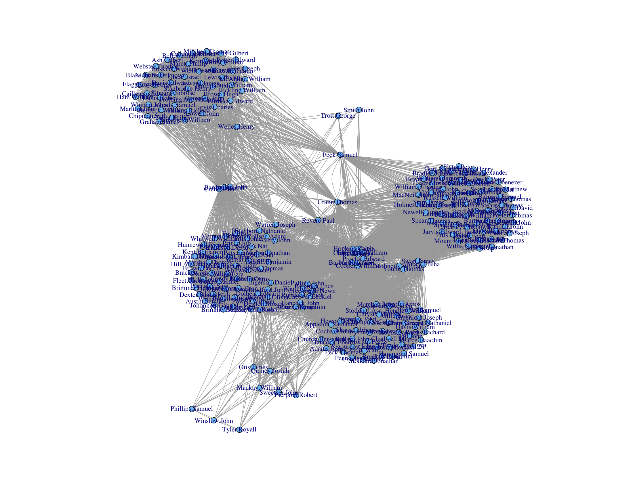
Constructing a graph based on historical data, Kieran Healy explains how we can use the graph to "find" Paul Revere.

I have been asked by my superiors to give a brief demonstration of the surprising effectiveness of even the simplest techniques of the new-fangled Social Networke Analysis in the pursuit of those who would seek to undermine the liberty enjoyed by His Majesty’s subjects. This is in connection with the discussion of the role of “metadata” in certain recent events and the assurances of various respectable parties that the government was merely “sifting through this so-called metadata” and that the “information acquired does not include the content of any communications”. I will show how we can use this “metadata” to find key persons involved in terrorist groups operating within the Colonies at the present time. I shall also endeavour to show how these methods work in what might be called a relational manner.

When to set office hours

This past term, I was assisting as a tutor for one section of a math course (I am teaching this course in the present term).  The students in the class wanted to have some extra tutorial time.  One of the students collected information about when everyone was available.  It turned out that there was no common period where all interested students could come, so there ended up being no extra tutorial.

This was between the professor and the students.  I didn't find out about it until after the fact.  I assume from the conversation, though, that there was going to be at most one extra tutorial, because the proposal was nixed once it was revealed that there was no common period.

But suppose that the professor was willing to offer a number of tutorials limited only by what periods where either he or I would have been available to lead one (assuming that the tutorials would be held during the day).  Then it may still be possible to find a way to accommodate everyone.  In fact, it's pretty easy to tell whether or not it is.

We already have a list of which periods students are available.  Since at least one of the available tutors (in this case, me and the professor) must be at the tutorial, we can strike from that list all periods where none are available.  If everyone is available in at least one of the remaining periods, then all students can be accommodated.  Otherwise it's not.

One way to do this is simply hold tutorials in each of those remaining periods.  However, professors have many responsibilities besides teaching ("publish or perish" and all that), so it's desirable to use the fewest tutorial periods possible.  So how can we do that?

It turns out that this is an application of a well studied problem in combinatorics, known as the set cover problem.  Suppose we are given a collection of sets, say $S_1,S_2,\ldots, S_k$.  Let $U=\cup_{i=1}^k S_i.$  Suppose that $I$ is a subset of $\{1,2,\ldots,k\}$ and $U=\cup_{i\in I}S_i$.  Then $I$ is called a {\em set cover} of $U$.  The set cover problem is to minimize the size of $I$.

Now, suppose that the periods are numbered $1,2,\ldots, k$.  For each $i$, let $S_i$ be the set of students who are available during period $i$.  Then the we can find the fewest tutorial periods needed by finding the smallest set cover of $U$.

Unfortunately, the set cover problem is NP-complete.  The formal definition of what this means takes a fair bit of work to explain, so I won't get into it here (if you're interested, follow the link to the topic in the Wikipedia article on the set cover problem).  In practical terms, though, it means that there is no currently known way to find the smallest set cover efficiently (and there probably won't ever be).  Perhaps the number of students and number of periods is small enough that it is still manageable by computer, or there is some approximation algorithm that will give a near-optimal solution.

Google "WordRank"

One of the more interesting things I learned about while I was a graduate student was Google's PageRank algorithm (to this day, it remains one of my go-to applications when I want to illustrate the real-life utility of certain concepts in linear algebra classes, although as each year passes, the likelihood that a student can remember life before Google gets smaller).  What made it particularly interesting to me is that it could be stated largely in the terminology of algebraic graph theory, my own field of research.  I had seen similar ideas before, but I had never seen anything like it put into practice (well, I had seen Google, but I wasn't aware that it was putting these ideas into practice).

The basic idea behind Google's algorithm is that good websites are websites that are linked to by good websites.  If you think that sounds awkwardly circular, you wouldn't be wrong.  Nevertheless, there's an elegantly simple way to express the idea as a matrix equation, and solutions to this equations are well studied.  Things don't always work out as well in practice as they do in the abstract, but Google's search engine was better than any search engines that came before it.  In this case, the abstract and practice lined up quite well.  In fact, the only one of these older search engines that's still around to this day in any noticeable way is Yahoo, but it has a much smaller share of the search engine market than Google does.

Now, one of my side interests is languages (or linguistics maybe, but I'm not sure how much my forays take me into actual linguistics. Favourite websites/blogs by people who know what they're talking about include Dialect Blog and Language Log).  While pursuing this interest, one of the things I've come across is lists of the most common words in a given language.  I wonder if something like Google's PageRank algorithm could be used to give an alternate word ranking words.  Instead of using links, you could say, in the same awkwardly circular fashion, that important words are words that are used with important words, set it up algebraically, then find the solution.  The result would assign a "WordRank" to each word.

What "used with" means is not well defined, mind you.  We could say that a word $A$ is used with a word $B$ if $A$ and $B$ are used in the same sentence, or perhaps used within a certain number of words of each other, regardless of whether or not they reside in the same sentence.  Maybe there is some other suitable choice.

While I could easily solve the algebra part, setting up the equation would take quite some work, and it might be beyond my abilities.  For example, if I chose to say words are used together when they are in the same sentence, I would need to decide whether or not a period in a given text is meant to indicate an abbreviation or the end of a sentence.  It's easy enough to do if I'm reading, but I would need to program a computer to do this for the a sufficiently large quantity of text.  That strikes me as a nontrivial task.

That wouldn't be a problem if I chose to say that words are used together when they appear within a certain number of words of each other.  Suppose this number is $n$.  The question arises as to what $n$ should be. The answer is not obvious to me.

Another complication is that spelling alone is not enough to determine what word is being used.  For one thing, words can have different forms.  Nouns can be plural or singular, verbs can be present tense or past tense, etc, and spellings change as a result.  Also, different words can have the same spelling.  There might be other issues (how to compensate for typos, maybe).  It would take some effort to sort these out, and I wouldn't know where to start.  These complications would crop up in producing lists based purely on frequency, though, and these lists already exist.  So I would assume somebody already knows how to deal with that.

Once these obstacles are overcome, we could make a matrix $M$.  The rows and columns of $M$ are both indexed by words (so the matrix is square).  If $v$ and $w$ are words, then $(v,w)$-entry of $M$ is the number of times $v$ appears with $w$ in some corpus.  Since $v$ is used with $w$ if and only if $w$ is used with $v$, $M$ is also symmetric.  Following the example of the PageRank algorithm, we find an eigenvector ${\bf x}$ of $M$ corresponding to the largest eigenvalue of $M$.  Provided that $M$ satisfies certain conditions, ${\bf x}$ will be unique up to a scalar multiple.  Furthermore, we can assume that the entries of ${\bf x}$ are all non-negative. (These are consequences of the Perron-Frobenius Theorem).  The vector ${\bf x}$ is called the principal eigenvector of $M$.  The entries of ${\bf x}$ can be ranked according to their size, with one entry ranked higher than a second if the first entry is greater than the second.  The WordRank of word $w$ is then the rank of entry $w$ of ${\bf x}$.

The total number of occurrences of the word $w$ is the row (or column) sum of row $w$ of $M$, which is given by $M{\bf j}$ where ${\bf j}$ is the all-ones vector.  Suppose that $D$ is the diagonal matrix where diagonal entry $w$ is the number of occurrences of word $w$.  Then column sums of $MD$ are all 1.  Since $M$ and $D$ are both nonnegative, $MD$ is as well.  Thus, $MD$ is a stochastic matrix, and therefore, the principal eigenvalue is 1.  As an alternative to the scheme derived in the previous paragraph, we could use the principal eigenvector of $MD$ instead of $M$ to determine a ranking.  The PageRank algorithm is based on the website analogue of this matrix.

In devising the PageRank algorithm, the Google founders found it necessary to modify this matrix further.   Perhaps some other modifications to $M$ or $MD$ would be necessary here.

One reason I think this could be interesting is that it's not just based on how common a word is, but how much each word "works" with other words.  The top $m$ words using WordRank could provide a more coherent list of words.  Of course, a word will get used more if it works well with other words, so any algorithm worthy of the name WordRank could end up producing more or less the same thing as ranking by frequency.

This idea could also be nonsense.  However, in the course of learning more about the PageRank algorithm, I came across another paper which generalized the algorithm.  In the paper, they applied a variation of  PageRank to the problem synonym extraction, with at least modest success.  So using these ideas in the realm of languages does not seem particularly absurd.

In any case, I think it would be interesting to see the results.

Possibly there are other things that could be done with the matrices $M$, $MD$, or maybe some other related matrix.  When designing language learning resources, it's important to come up with vocabulary lists.  We could use frequency or WordRank, or some combination, to compose a these lists.  But these lists probably need to be divided into smaller chunks for individual lessons.  One would hope that these chunks consist of a coherent set of words, for example, words centred on a theme, like food related words, occupation related words, and so forth.

One could do this by hand, of course, and maybe that's the best way once you decide which words to use.  But there are techniques based on eigenvalues and eigenvectors (for example, using the Fiedler vector) that are used to subdivide networks into smaller coherent components.  Perhaps some variation of these techniques could be employed here.

A graph labelling problem

I've been doing some work using the shapefiles for the current Canadian federal electoral districts.  Each shape in the shapefile corresponds to a riding (or, in a few cases, a part of a riding).  One thing I have noticed while working with them is that there is no apparent structure to the order in which the shapes appear.

For example, Shape 1 is the boundary of the Vegreville--Wainwright riding in Alberta, while Shape 2 is Bruce--Grey--Owen Sound in Ontario.  Since Alberta and Ontario do not even share a border, these two districts are far apart from each other.  Meanwhile, the ridings adjacent to Vegreville--Wainwright are numbered 5, 21, 144, 183 195, 217, and 240.  Considering there are only 312 shapes [1] in total, 5 and 21 are the only numbers remotely close to 1.  If there is any reasoning behind the numbering scheme, it's not easy to tell what it is by looking at the numbers alone.  One assumes it's arbitrary.

I use the numbers frequently, so it would be helpful if I could tell a little bit more about how close two ridings are based on their numbers.

The best numbering system would have consecutive numbers mapped to adjacent ridings, so that one riding was adjacent to another if and only if their labels differed by exactly 1.  This impossible to do for every riding, however, since it would require each riding to be adjacent to only two other ridings, but most are adjacent to three or more others.

Instead, we could number the ridings so that the numbers of  ``close'' ridings are also close.

There are a couple ways we could do this.  First, let's put the problem in terms of graph theory.  Let $G$ be the graph whose vertices are the electoral districts.  Define two vertices to be adjacent if their corresponding districts share a border (excluding the case where two districts share a point).  Suppose we label each vertex $v$ with a number $n(v)$ between 1 and the number of vertices, using each number for exactly one vertex.

1. Ensure adjacent vertices have close numbers.  Thus, for each pair of adjacent vertices, compute the difference between their labels, then take the sum of these numbers over all adjacent pairs.  That is, compute
   $$\sum_{uv\in E}|n(u)-n(v)|$$
   Define the best labellings to be those that minimize minimize this sum.
2. Approximate the the distances between vertices with the difference between their respective labels.  To this end, let $d(u,v)$ be the distance between two vertices in the graph and let $D(u,v)=|n(u)-n(v)|$.  The difference between the labels approximates the distance between the vertices if $|d(u,v)-D(u,v)|$ is small.  Thus, define the best labellings to be those that minimizes the sum
   $$\sum_{uv}|d(u,v)-D(u,v)|$$

The first approach bears some similarity to the graph bandwidth problem.   In the bandwidth problem, the goal is to minimize the maximum value of $|n(u)-n(v)|$.  If this value is $m$, then $m|E|$ is an upper bound on the sum that appears in the first approach.  It's possible, however, that the sum and the maximum are minimized by different labellings. 

The fact that the graph bandwidth problem is NP-hard suggests that it will also be difficult to minimize the sum.  I also suspect that the sum in the second approach will be of comparable difficulty.

Edit: One way of interpreting the graph bandwidth is not obvious from the name (the name is derived from matrices associated with the graph).  If we think of the labels $n(v)$ as locations of vertices along the line from 1 to $|V|$, then $|n(u)-n(v)|$ is the length of the edge.  So the graph bandwidth is the smallest possible value for the length of the longest edge.   We can say something similar about the first solution.  The goal in that case is to minimize the total length of the edges, or, equivalently, the average edge length.

[1] The astute reader will notice that there are 308 ridings in total for the last election, and there will be 338 in the next.  So where does this 312 come from?  Two ridings include islands that are too far from the mainland to be included in the same shape, so are included as separate shapes, and one riding includes 3 mainland components that are separated from each other by another riding, yielding 4 extra shapes.

Antiderivative vs. Indefinite integral

I spent some time today getting ready for my class for the next term.  In particular, I was reading through the sections on antiderivatives and indefinite integrals.  I had normally taken these things to be distinct concepts.  Given a function $f$, an antiderivative of $f$ is any function whose derivative is $f$.  The indefinite integral is the set of all antiderivatives.  Since there are infinitely many antiderivatives, while an antiderivative is a single function related to $f$ by differentiation, these are not the same thing.

Or at least, that's what I thought until I read the aforementioned sections. The definitions I read today did not seem to make that distinction.  I consulted with the textbook that I used in my own first year calculus class many years ago.  This textbook does make the distinction.

I suspect the difference between the two ideas is not appreciated by a lot of students.  We don't dwell on it much once we give the definitions.  After that, we usually teach them techniques for finding indefinite integrals, and as long as they remember to include the constant of integration, we're happy.

The textbook that doesn't distinguish the two is one of the most widely used introductory calculus texts.  It's quite an old version, though.  Perhaps newer versions do distinguish.

In any case, it made me wonder how important, if at all, the distinction is.  Was a serious error made by leaving it out?  Am I being too picky by insisting my students understand the difference?

One thing I do find somewhat bothersome about erasing the distinction is the abuse of notation that results.  If $F$ is an antiderivative of $f$, then it can be written
$$\int f(x) dx = F(x)$$
The constant of integration is omitted because there is no distinction between the two terms.  This is an abuse of notation, because there are actually infinitely many functions that could appear on the right, all differing form $F$ by a constant.  So the $=$ sign doesn't belong there, because it implies uniqueness.  Of course, even writing the constant of integration
$$\int f(x) dx = F(x)+C$$
can be seen as an abuse of notation, but at least it captures the idea that there are infinitely many antiderivatives of $f$ and each of them has the form on the right.  I suppose, to capture the essence of the idea, we could instead write
$$\int f(x) dx = \{F(x)|F'(x)=f(x)\}=\{G(x)+C|C\in{\mathbb R}\}$$
where $G$ is a known antiderivative of $f$, but I've never seen it written this way.

Expansion Minimization

The determinant of a square matrix $A$ is typically defined in terms of cofactor expansion along the first row of $A$.  Then cofactor expansion along other rows or along columns is defined, and shown (or stated) to be equal to the determinant.  Following that, there is usually an example of a matrix that contains at least one zero.  This example is used to illustrate that sometimes, if we choose the appropriate row or column to expand along (namely, one with zeros), we can reduce work needed to compute the determinant using cofactor expansion.

It is certainly easy to tell which row(s) or column(s) to expand along to minimize the number of cofactors it is necessary to compute at each step.  Simply expand along a row or column that has the most zeros.

But what row or column should we expand along to minimize the total number cofactors to compute overall?  Or, to put it in more practical terms, what row or column should we expand along to minimize the
 amount of writing necessary?

Something to consider is that there are two ways to get a zero in the cofactor expansion.  If $B$ is some square submatrix encountered in the cofactor expansion of $A$, then either $b_{ij}=0$ or $\det B_{ij}=0$ ($B_{ij}$ being the $(i,j)-minor of $B$) to make a cofactor.  Since determining whether or not $\det B_{ij}=0$ requires a determinant computation, we would probably want to know the answer to the question to answer the question, which leads to circular reasoning.  So we'll assume that we're basing our expansion minimization strategy purely on which entries of $A$ are 0.

Of course, the answer to the question posed here is mostly useless for practical purposes, since nobody is going to compute the determinant through cofactor expansion for all but the smallest matrices.


But since we frequently present these example and pose these problems to students, with the expectation that they'll know what the best row or column is to expand along, I wonder if there's actually some way to tell what the best path to the determinant is from the matrix itself.

A Few Questions Related to Planar Eulerian Graphs

Let $G$ be an Eulerian graph.  Suppose there is some planar embedding of $G$ in the plane.  When does $G$ have a "non-crossing" Eulerian cycle?  That is to say, if there is a planar drawing of the graph, when can we find an Eulerian cycle in the graph that can be drawn along the edges of the planar drawing without crossing itself?

More generally, suppose that $G$ has $2t$ pairs of odd-degree vertices.  It is known that the edges of $G$ can be decomposed into $t$ paths.  When is there a set of $t$ paths that decompose the edge set of the graph and that can be drawn without crossing themselves or each other?

Even more generally, suppose that $G$ has an embedding into a surface of genus $g$ (or non-orientable genus $g$).  When is there a set of $t$ paths that decompose the edge set of the graph and that can be drawn without crossing themselves or each other?

Planar Graph Drawing Problem

Suppose that $G$ is a planar graph.  Define a convex representation of a graph to be an assignment of each vertex $v$ in $V(G)$ to a convex polygon $p(v)$ so that two vertices $u$ and $v$ are adjacent if and only if $p(u)$ and $p(v)$ intersect only on their boundaries in at least one edge (i.e. so that the polygons share more than just vertices, but the area of their intersection is zero).  Furthermore, suppose that each vertex $v$ in $V(G)$ is assigned some positive number $f(v)$.

Does there exist a convex representation of $G$ so that the area of polygon $p(v)$ is equal to $f(v)$ for all $v$ in $V(G)$?

If $G$ is not 3-connected, then the answer is no, since a graph has a convex representation if and only if $G$ is 3-connected.  An algorithm due to Tutte, applied to the dual graph, will find a convex representation, though it might not be aesthetically pleasing.

Based on the number of area cartograms that have popped up lately, it seems that representation of the graph by polygons with specified areas is also possible, if not all of the time, then most of the time (I've never seen a theorem to that effect, though it does seem plausible).

What asking for, then, is the intersection of both of these ideas.  Like the Tutte embedding, the representation should be convex.  Like the area embedding, the areas of each polygon should have the same size.

Variable x, Ex-variable.

Is the variable $x$ still a variable once a value has been assigned to it?  Because then, $x$ is fixed at the assigned value and can no longer vary, and that which cannot vary is not variable.

Coefficient Operation

The trace of a matrix satisfies the following equation
$$tr(A+B)=tr(A)+tr(B)$$
The trace is also the coefficient of the second highest power of the characteristic polynomial (up to a factor of $-1$).

The determinant of a matrix satisfies the following equation
$$det(AB)=det(A)det(B)$$
The determinant is also the constant term of the characteristic polynomial (up to a factor of $-1$).

Thus, for both the trace and the determinant functions, there is a binary operation that is defined for both matrices and numbers, and the functions distribute over the corresponding binary operations.  Furthermore, both functions appear in the characteristic polynomial.

If the matrix is 3x3 or larger, then there are many coefficients between that of the determinant and that the second highest power.  We can think of these as generalizations of the trace and determinant.

That is, suppose that $f_k(A)$ is the coefficient of $\lambda^k$ in the characteristic polynomial $p(\lambda)$ of the $n\times n$ matrix $A$.  Then $tr(A)=f_{n-1}(A)$ and $det(A)=f_0(A)$.

That leads to the following question.  For each of the $k$, does there exist a binary operation, say $\circ_k$, that is defined for both square matrices and numbers such that $f_k(A\circ_k B)=f_k(A)\circ_k f_k(B)$ (up to a factor of $-1$)?  Note that we want $A\circ_k B$ to be a matrix and $a\circ_k b$ to be a number.

We can take $\circ_{n-1}$ to be the trace function and $\circ_0$ to be the determinant function, so the answer is yes for $k=n-1$ and $k=0$.

The coefficient of $\lambda^n$ is always $\pm 1$.  Define $\circ$ by $a\circ b=1$ and $A\circ B=I$.  Then $f_n(A\circ B)=f_n(I)=1$ and $f_n(A)\circ f_n(B)=1\circ 1=1$.  Thus,
$$f_n(A\circ B)=f_n(A)\circ f_n(B)$$
So we could take $\circ_n$ to be the binary operation $\circ$ defined here.  So the answer is yes for $k=n$ as well.  Note that $a\circ b$ must be defined to be 1 in order to satisfy the desired property, but $A\circ B$ could be defined to be any matrix, since $f_n$ is always $\pm 1$. 

What can be said about $\circ_k$ for $k\in\{1,\ldots,n-2\}$?

There was some freedom in how we defined $\circ_n$.  It is not unique.  Is this true about the other $\circ_k$, if they even exist?

Two Videos

A friend sent me the following video today, inspired by a child's toy.

I've come across similar statements about things being "countless", and also cocked an eyebrow when I heard them. For example, I once read that postal codes were unlimited as well, when there are, in fact, only 17,576,000 different possibilities, roughly half of the number of people in Canada. In any case, it never occurred to me that such dubious claims (well, dubious to the mathematically trained) could be turned into lessons. It's quite remarkable just how interested the students got in the problem. This video, enticingly titled "998,001 and its Mysterious Recurring Decimals", showed up as one of the recommended videos in the sidebar.

The topic of this video would make an interesting diversion in a course on infinite series, and like the previous video, it has something of a combinatorial flavour.

David Gregory

[Updated: see below]

On Thursday afternoon, I received an email from one of my colleagues that my former supervisor David Gregory's cancer had progressed and that he was in palliative care.  I originally planned on visiting him the next day on Friday.  However, I ended up spending most of the day finishing up a job application that was due shortly, and the tone of the email did not suggest the situation that was that dire.  I had commitments on the weekend, so I put off the visit until Monday.  On Monday morning, though, I received an email from Kevin Vander Meulen, friend, fellow collaborator, and also former student of David, who had found his obituary:

GREGORY, David - David Gregory of Kingston, Ontario passed away peacefully on Friday July 12, 2013 with friends and family by his side. He is predeceased by his parents Alan and Edith (Towell) Gregory. He is survived by his sister Betty Jane Lerer (Gregory) and his brother-in-law Harvey Lerer. As well he is survived by his nephew Michael Lerer, his niece Tara Lerer (Middleton) and great-nephew David Lerer. The family wants to thank his many friends and colleagues for their care and sympathy throughout his illness. A private funeral is arranged. A memorial celebration of David's life will be held in the near future. In lieu of flowers, donations to The Canadian Cancer Society or the University Hospitals Kingston Foundation would be preferred.

Even if I had gone on Friday, it might have already been too late.

The first time I had seen David speak was when he gave a guest lecture on the Good Will Hunting Problem to my undergraduate graph theory class.  Although I would not meet him until a few years later, I worked with David for the first time in the spring/summer of 1999 between the 3rd and 4th years of my undergraduate studies on the problem of addressing the Petersen Graph, the graph after which this blog is named.  I would collaborate with him again the following summer.

It wasn't until the fall of 2001, when I had started my master's degree at Queen's University, that I met him for the first time.  He was already retired then, after his first bout with cancer.  Although he was still clearly recovering from his treatment, he would still regularly come into his office to work on his research.

After that, I didn't speak with him again until my original supervisor, Dom de Caen, had passed away in the spring of 2002.  Even though he was already retired, David happily accepted me as his master's student, and later as his PhD student.

David was very dedicated as a supervisor.  We met at least once a week, sometimes briefly, and sometimes for a whole afternoon.  If I had questions outside of our regularly scheduled meetings, he was always happy to make time to discuss them with me, even if I just showed up at his door.  When I reflect on the quality of the first draft of my master's project, I can't help but conclude that he was a very patient man.  He helped me to turn what was a very rough draft into the final draft, without ever letting on that I had burdened him in any way.  He demonstrated the same patience and dedication throughout my PhD studies as well, being available early in the morning as well as sending me helpful emails late in the evening.

David was a regular participant in the Discrete Math Seminar held jointly between the respective departments at Queen's University and the Royal Military College, which I frequently attended.  His talks were always interesting, well organized, and easy to follow.

In addition to his role as a supervisor, he was also a good friend, giving me advice on personal matters and helping in other ways.

He will be missed.

-----

A memorial page has been set up by Bryan Shader, one of David's friends and collaborators.

Why iPod Shuffle isn't Random (Updated)

(Updated, see below)

The idea for this post came from a book that I picked up and put down at a  Chapters/Indigo store some time ago.  I don't recall the title or author of the book, unfortunately.  I've gone to both locations in town to find the it back again, but can't.  So instead I'm going to try to recreate the argument that I didn't have time to read in full when I first saw it.

One thing I do recall from the book is that Apple got a bit of bad press because people didn't think their randomization algorithm was truly random.  The time it took to hear a repeat was too short according to listeners.  Suppose for example, that I have 100 tracks on my iPod.  Then shouldn't I hear each track once in every 100 tracks?  On average, yes.  If the selection is truly random and I listen to enough tracks consecutively, then the average gap between each repeat of that track will be 100 (or 99, depending on whether or not you count the second occurrence towards the gap length).

However, the average doesn't describe what always happens, just what happens overall.  It's possible, although unlikely, for the first two tracks to be the same, so we get a repeat right away.  It's also possible, although very unlikely, to be able to listen to all 100 tracks straight, without a single repeat, so we don't get our first repeat until the 101st track.

Note that we must have a repeat by track 101.  For suppose that we listened to 100 tracks straight with no repeat.  Then we have heard all 100 tracks.  Thus, the 101st track must be a repeat.  This is an application of the  Pigeonhole Principle, where each track is a "pigeonhole" and there is one "pigeon" in it for each time we hear the track.  Therefore, we only need to concern ourselves with the chance of a repeat in the first 101 tracks.

We'll answer the question of the average time before a repeat in stages.  First we'll determine the probabilities that the next track is or isn't a repeat, assuming that no repeats have occurred.  Next we'll determine the probabilities that the first repeat occurs at track 1, track 2, etc.  Finally, we'll use these to calculate the average track number at which the first repeat occurs.

Probability that the next track is a repeat
First, we consider the probabilities of a repeat and non-repeat, assuming that previous track is not a repeat.  Obviously, there is a $0\%$ chance that the first track is a repeat, because there are no tracks before it that it can be a repeat of.

After listening to the first randomly chosen track, there are 99 other tracks that we haven't heard.  Since each track is equally likely to occur, the chance that the second track is same as the first is $\frac{1}{100}$, and the chance that it is different is $\frac{99}{100}$.

Suppose that the first two tracks are different, i.e. that the second track was not a repeat.  There are now 2 tracks we have heard, and 98 that we haven't.  Thus, there is a $\frac{2}{100}$ chance that the next track is a repeat and a $\frac{98}{100}$ chance that it is not.

Similarly, if there is no repeat by the 3rd track, then there is a $\frac{3}{100}$ chance that the next track is a repeat and a $\frac{97}{100}$ chance that it is not.  If there is no repeat by the 4th track, then there is a $\frac{4}{100}$ chance that the next track is a repeat and a $\frac{96}{100}$ chance that it is not, and so on.

In general, if we have listened to $k$ tracks without a repeat, then the chance that the next track is a repeat is $\frac{k}{100}$ and the chance that it is not is $\frac{100-k}{100}$.

Probability that a specific track is the first repeat

The next things we need to know are the chances that we will hear the first repeat at track 1, track 2, track 3, etc.

The chance of hearing the first repeat at txrack 1 is 0, as explained above.  The chance of hearing the first repeat at track 2 is $\frac{1}{100}$.

In order to hear the first repeat at track 3, tracks 1 and 2 must be distinct, and track 3 must be the same as either track 1 or 2.  As explained above, the probability that 1 and 2 are distinct is $\frac{99}{100}$ and the probability that 3 is the same as 1 or 2, assuming 1 and 2 are distinct, is $\frac{2}{100}$.  Thus, the probability that the first two tracks are distinct but the third is the same as one of the first two is
$$\frac{99}{100}\frac{2}{100}$$
In order to hear the first repeat at track 4, tracks 1 through 3 must be distinct.  The probability that second track is different from the first is $99/100$ and, assuming the the first two are distinct, the probability that the third is also distinct is $98/100$.  Thus, the probability that the first 3 tracks are distinct is
$$\frac{99}{100}\frac{98}{100}$$
Since the first three tracks are distinct, the probability that the fourth track is a repeat is $3/100$, so the probability that track 4 is the first repeat is
$$\frac{99}{100}\frac{98}{100}\frac{3}{100}$$
Similarly, the probability that track 5 is the first repeat is
$$\frac{99}{100}\frac{98}{100}\frac{97}{100}\frac{4}{100}$$
In general, the probability that the first repeat happens at track $k$ is
$$\frac{99}{100}\frac{98}{100}\cdots \frac{(100-k+2)}{100}\frac{k-1}{100}=\frac{(k-1)99!}{100^{k-1}(100-k+1)!}$$

where $n!=n(n-1)(n-2)\cdots (2)(1)$ (read "$n$ factorial")

Average track of the first repeat

To get the average track number at which the first repeat happens, we multiply each number $k$ between 1 and 100 by the probability that the track $k$ is the first repeat, then add the results.  That is, the average track number for the first repeat is
$$0(1)+\frac{1}{100}(2)+\frac{99}{100}\frac{2}{100}(3)+\frac{99}{100}\frac{98}{100}\frac{3}{100}(4)+\cdots+\frac{(101-1)99!}{100^{101-1}(100-101+1)!}(101)$$
It's far too much work to calculate this number by hand, but plugging this into a computer  gives track 13.21 (rounded to two decimal places).  So we can expect to get through only a small fraction of my music collection before we start to hear repeats.

If we use the average length of a pop song of between 4 and 4.5 minutes, that means we can expect to hear the first repeat at somewhere between 53.8 minutes and and 59.4 minutes.

The other averages
Typically when we talk about average of some values, we mean the mean, i.e. the sum of the values divided by the number of values.  There are other types of averages, though.  The median and the mode are probably the most common. You probably learned about them in school, but forgot about them because they're not as widely used, although they are sometimes situations where one of them might be more suitable.

The median, for example, is the middle value (if the numbers are ordered).  For example, suppose our values are $1,2,2,3,4$.  There are 5 values in total, so the third value is the middle value.  Therefore, the median of this list of values is 2.  The median is preferable to the mean when talking about average incomes, because the very small number of people with very large incomes drives up the mean, giving a skewed perception of the typical income.  The median, on the other hand, is more stable.  For example, the $4$ could be changed to $40$ or $4,000$, but the medians in both cases would still be 2, while the means change to 9.6 and 801.6 respectively.

The mode is the most frequently occurring value.  In each of the lists of values in the preceding paragraph, the number $2$ appears twice, while each other number only appears once, so the mode is 2.  The mode is useful when our values aren't numbers.  For example, you could take a poll on people's favourite colour.  The mode is the colour that is picked by the most people.  The median and the mean are not defined in this case, because colours are not numbers (they can be described numerically, but the numerical description would not be of much use in this case).

A more detailed discussion on mean, median, and mode can be found here.

The median for number of tracks before a repeat in this case is 12 or 13.  This means that roughly half of the time, the first repeat will occur on or before the 12th track, and roughly half of the time, the first repeat will occur on or after the 13th track.

The mode in this case is 11.  That means that the first repeat happens at track 11 more often than it happens at any other track.  The probability that it will happen at track 11 is quite small at only 6.28\%. However, the probability that it will happen at any other track is even smaller (and the further from 11 we get in either direction, the lower the probability is).

Conclusion

All three of these averages are pretty close to each other, relative to the size of the music collection, and they all represent a pretty small fraction of the collection.  To make matters worse, more than half the time, a repeat is going to happen before the average.

Now, a music collection of only 100 tracks is rather small.  My own currently has around 400 tracks, and I'm not even an avid purchaser of music.  The mean track number of the first repeat for a 400 track collection is 25.73, the median is 24, and the mode is 21.  Thus, the different averages just barely double (if that), even though the music collection is 4 times as large.

If we multiply by 4 again, for a collection of 1,600 tracks, the mean is 50.8, the median 48, and the mode 41, again, roughly only doubling the number of tracks before a repeat.

Thus, even for large collections, no matter how much Apple made sure that tracks were chosen randomly, we would be bound to hear repeats after only a small proportion of the tracks.  So we don't actually want true randomness.  Apple solves this problem by choosing a fixed ordering of the tracks each time the iPod (or iPhone, iTunes, etc) is started, much like shuffling a deck of cards, thus the name "shuffle".

Admittedly, I'm using a bit of verbal sleight of hand here, taking advantage of the ambiguity of the word "random".  There is an element of randomness in the shuffle too.  After all, the category of games of chance includes games played with a shuffled deck of cards.  To form the list, the first track can be chosen at random from the collection, and each subsequent track can be chosen randomly from the tracks that haven't been chosen yet, but this is not typically what's meant by the word "random" when it appears without any qualifiers.

Despite Apple's attempts to fix the problem, however, there are still skeptics.

Update.  It's been about a year since I first wrote this.  I never did find the book that I referred to above.  However, I did find a related problem in another book called Duelling Idiots and Other Probability Puzzlers by Paul Nahin.  In one of the latter chapters, the author discusses the NBA draft where a similar problem shows up.